This looks long, so what’s the TLDR version of what you found?
Using games from 2020 in which at least two running backs from a team had at least 5 carries, the yards per rush attempt of each game were compared between running backs to see the degree to which the “best” running backs in the league generate more yards on a given rush compared to their backups.
When comparing the running back who led their team in rush attempts to every other running back on the team, there was no meaningful difference in yards per rush attempt between starting and backup running backs (i.e. Le’veon Bell and Bilal Powell would not be expected to differ consistently in yards per carry in games where they both had at least 5 carries). Additionally, the best predictor of rush yards per attempt on a game-by-game basis was the opposing team’s season grade for rush defense as provided by Football Outsiders.
Given this, if the hope is to maximize yards per carry, then there doesn’t appear to be much need to pay a premium for running backs.
Why are you bothering to examine this?
The value of running backs was never really questioned prior to the rise of analytics. Indeed, a glance at the hall of fame and lists of the best football players ever feature tons of running backs. And why wouldn’t they? Few things are more fun or memorable on a football field than watching a defense look helpless when guys like a prime Chris Johnson blur past an entire team or when guys like Marshawn Lynch bowling ball their way down the field as defenders fall off of them. However, in recent years, the question of the value of running backs has been raised and a notable amount of data has supported that individual running backs don’t really matter all that much and that the perceived value that they are assigned comes from their offense line and the team around them rather than innate talent.
As Jets fans, I think it’s kind of hard to not be aware of this new line of thought and to at least give it some consideration as the team recently gave Le’Veon Bell a 4 year, 52 million dollar contract just to watch his yards per rush attempt plummet from a solid 4.0 with Pittsburg in 2017 to 3.3 with the Jets in 2019. This then begs the question, is it Bell? Did his talent freefall off a cliff? He did take a year off prior to joining the Jets, so, maybe? Or is it that the Jets and their offensive line are really bad compared to what Bell had in Pittsburg and that Bell the player hasn’t changed much even if his stats have? With these questions in mind and inspired by a debate on this lovely site of ours, I decided to dig into it myself. What follows, is what I found and how I found it. To make things a bit more digestible I broke it up into questions.
How did you go about examining this?
Part 1: What data did you collect?
While the idea started out small, it kind of just kept building, so I’m going to walk through in terms of where I started and where I ended chronologically.
At first, my goal was simply to examine the yards per rush attempt of different running backs who ran behind the same offensive line against the same defense. My thought being that if we keep constant the offensive supporting cast and the defensive opponent then we could figure out what a guy like Bell adds over a guy like Powell. This is thought to be examinable because as we control for other variables (i.e. the shared quality of the offensive line), then the variable we change (i.e. the guy running the ball) is more likely to actually be the cause of any difference. In this case, I was interested in yards per rush attempt because that helps us to compare how efficient on a given run a guy like Bell, who received 200+ carries this year, is to a guy like Powell, who only received 40 carries this year.
To that end, I scoured the internet until I found a dataset that a) had the data I needed and b) was easy to access. The site I wound up settling on was fftoday.com, which provides stats by position for each week of the NFL season. Using that site, I was able to pull the stats for all running backs for each of the 17 weeks. From there, I pooled all of that data into one sheet, which contained the name, team, rush yard per attempt, number of rush attempts, and the week in which the game was played. Additionally, I decided to only keep the data when running backs had at least 5 carries as anything less than that felt like capitalizing on chance given that having 1 rush for 20 yards for an average of 20 yards is possible with one carry, while that average is not really feasible for a guy who carries the ball 10 or 20 times. Admittedly, 5 was an arbitrary cutoff, but I think it was better than nothing.
Following this, I decided that simply analyzing those few stats was not enough to tell a thorough enough story. At this point, I started to think about other variables that might be relevant. After some time, I wound up settling on adding QB data for each game as well as opponent defensive data for each game. In order to cull this data, I used fftoday.com to grab QB stats and footballoutsiders.com for their DVOA statistics. For those of us that aren’t familiar with DVOA, it essentially assigns a percent value to the defense based on their performances relative to the average and is interpreted such that more negative scores are better than more positive scores. The variables that wound up being of interest to me on defense were rush defense DVOA and pass defense DVOA as I felt that this captured each facet of the defense and, together, was pretty encompassing of overall defensive performance. For QBs, I was interested in yards per pass attempt, number of pass attempts, yards per rush attempt, and number of rush attempts by the QB, specifically. I figured these statistics covered the rate at which these plays were occurring and also how valuable the average play was. Also worth noting, as it wasn’t uncommon that QBs ran 0 times for 0 yards, so I changed those yards per attempt values to be 0 with my thought being that the goal of yards per attempt in this analysis was to gauge the risk that a defense had to concern itself with a QB running on a given play and a guy who doesn’t run has a risk of 0.
Lastly, given that my aim was to compare running backs from the same team within the same game, I opted to remove teams where a running back that didn’t lead the team in carries did not register at least 5 carries in at least one game. As I found out, three teams accomplished this (Carolina Panthers, Oakland Raiders, and Jacksonville Jaguars), so they were removed.
Part 2: What data did the data look like?
After taking all of these datapoints into account and logging them, I was then able to put to them in one large dataset. After all of this is when the fun begins with data and pretty visuals.
First, I wanted to plot what I was looking at in terms of yards per rush attempt. To accomplish that, I did a few things.
One, I plotted the frequency for which players ran for an average of 1 yard per rush attempt, 2 yards per rush attempt, etc. For ease of interpretation, all of these were binned such that a
rush of 1.1 and a rush of 1.4 were both logged as being 1, and a rush of 1.5 and 1.9 were both logged as 1.5 yards per rush attempt. This data looked like the following:
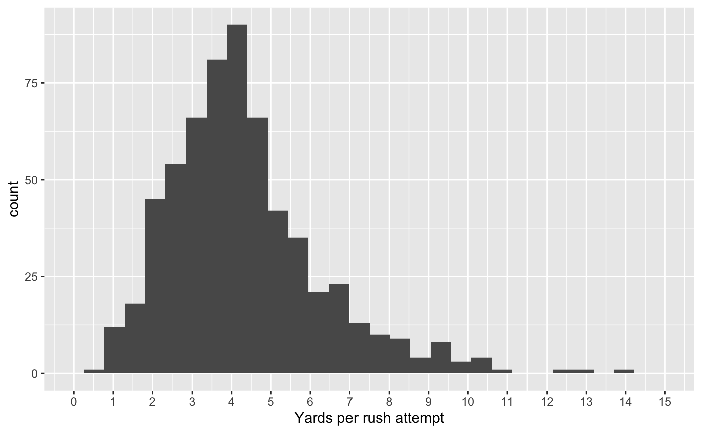
Note, I was a bit concerned about those values that were greater than 10 as that felt like it might be capturing too much on chance with guys who had exactly 5 rushes and happened to rip off a big one. However, I then went in and looked at those 9 datapoints and opted to keep them after seeing that the lowest number of rush attempts was 8, which felt like enough to me to be an accurate account of how well a player played on that day, so I opted to keep them all.
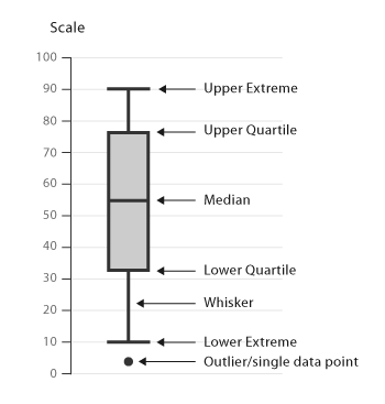
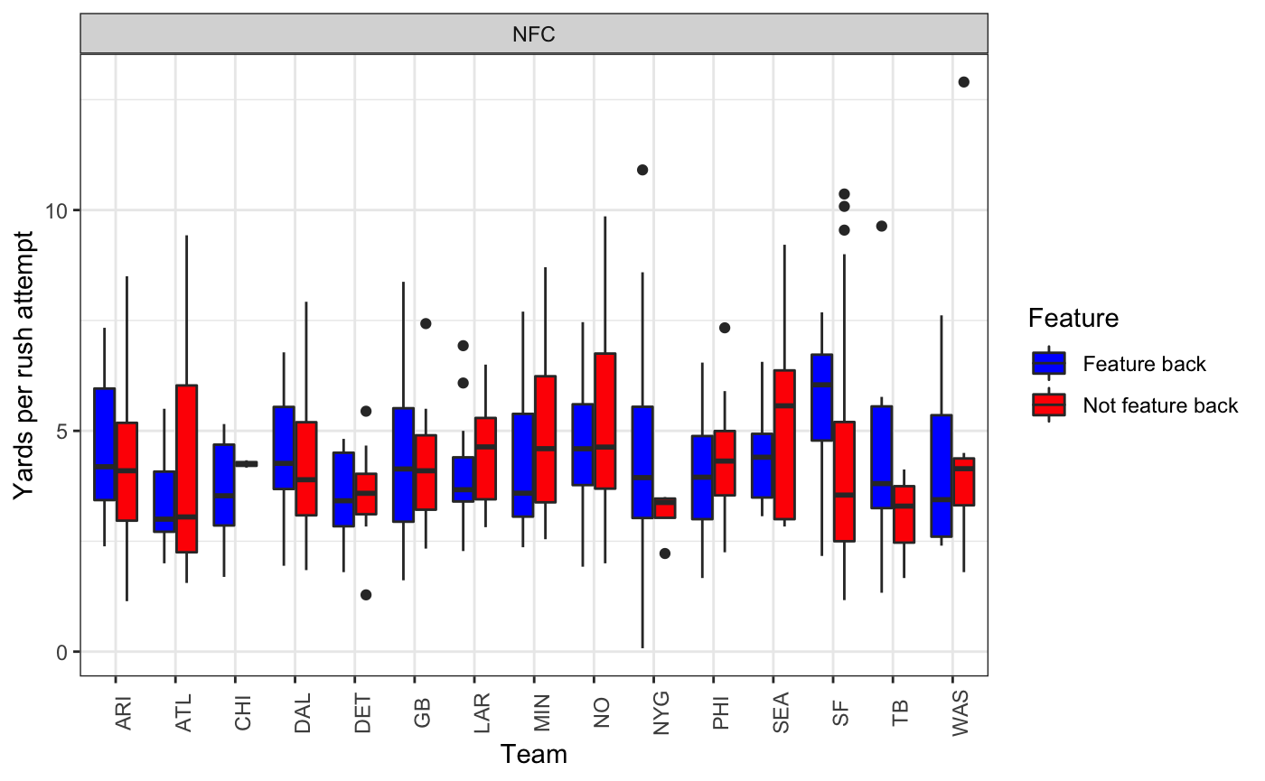
Two, I plotted the yards per rush attempt by team. I wanted to get a gauge for how much these median values differed between teams (i.e. were the Jets averaging 3 yards per rush attempt while everyone else averaged 6?) and how much they differed within teams (i.e. was every running back on the Jets averaging 3 yards per rush attempt or was Bell running for noticeably more?). To do that, I created box-and-whisker plots. For those of us that aren’t familiar with box-and-whisker plots, I pulled this handy visual primer from https://datavizcatalogue.com/methods/box_plot.html
With that said, I created the box-and-whisker plots that follow and will provide a brief explanation of what the big takeaway from each plot is
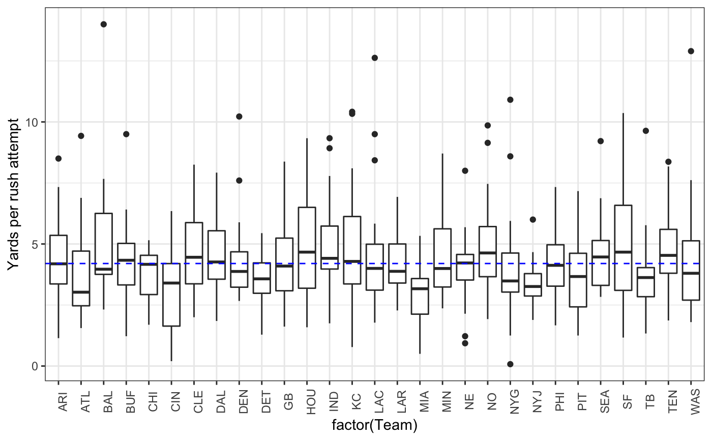
Pay attention to the thick black line in the middle of the white boxes as this notes the median, which is the 50th percentile for the variable of interest. As you can see, the medians are pretty consistent across teams with most of the hovering right around 4.3, which gives us an early indication that rush yards might not vary as much between teams as I thought. To further show this, I added a blue dashed line at 4.3 that runs horizontally through the graph.
Also, of note as Jets fans, the Jets are one of the fewer teams that appear to be meaningfully below that line, which I don’t think will surprise any of us.
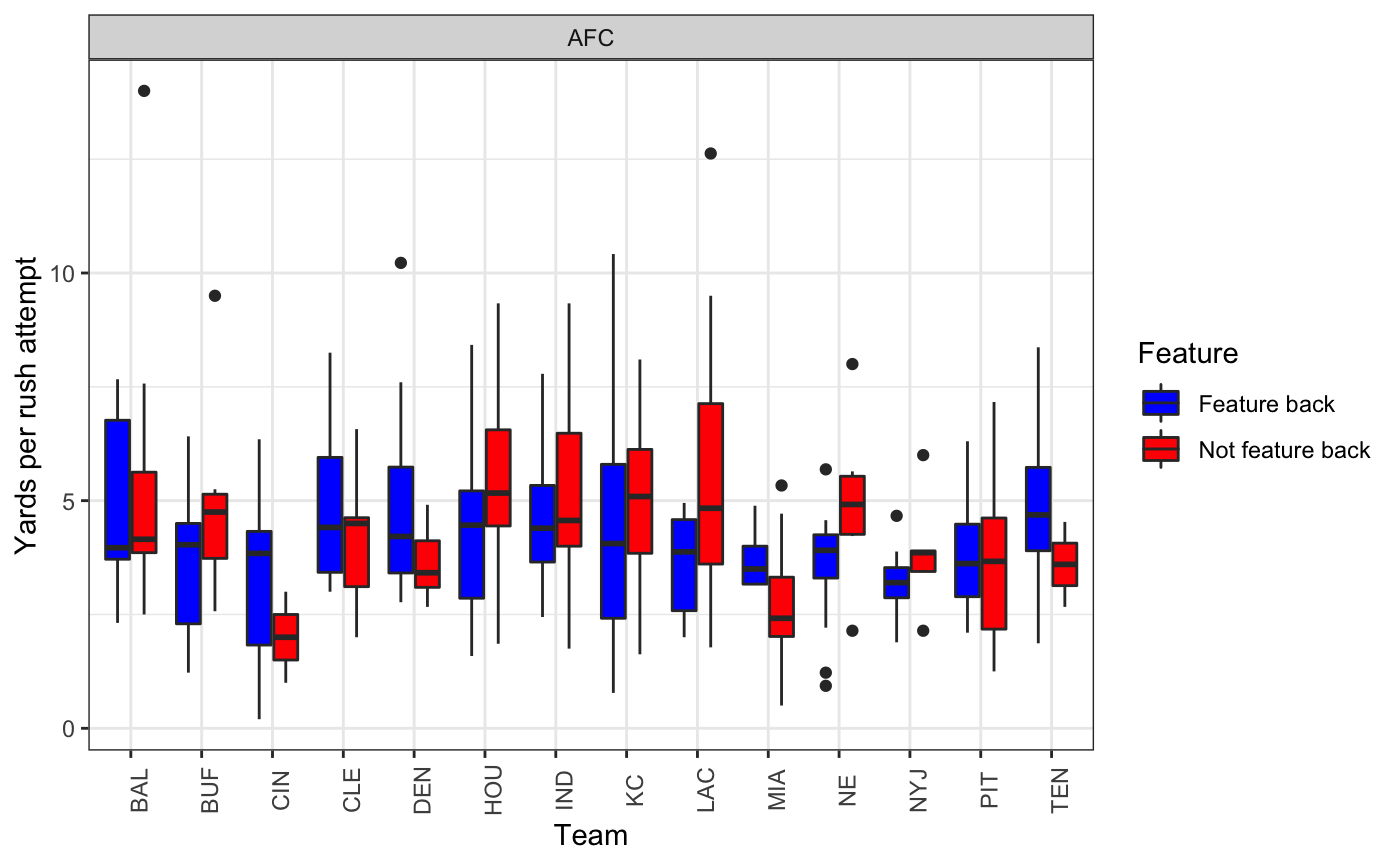
In this graph, I separated the team leader in rush attempts (labeled as Feature back) from all other backs on the roster (labeled as Not feature back). As you can see, there’s a decent amount of variation in how these two groups did within team, which is good as this gives us an early sign that we might be onto a difference. The problem is that there doesn’t appear to be a clear pattern with some teams having the feature back (shown in blue) having higher medians and box placements than the other backs (shown in red) and others showing the reverse. In order to make sure the graph wasn’t too bunched, I opted to create one graph for the AFC (shown above) and another for the NFC (shown below).
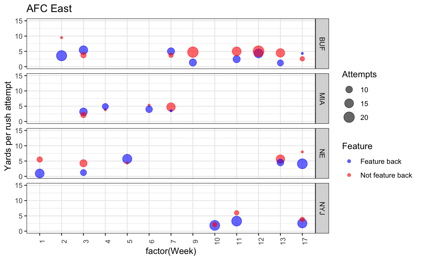
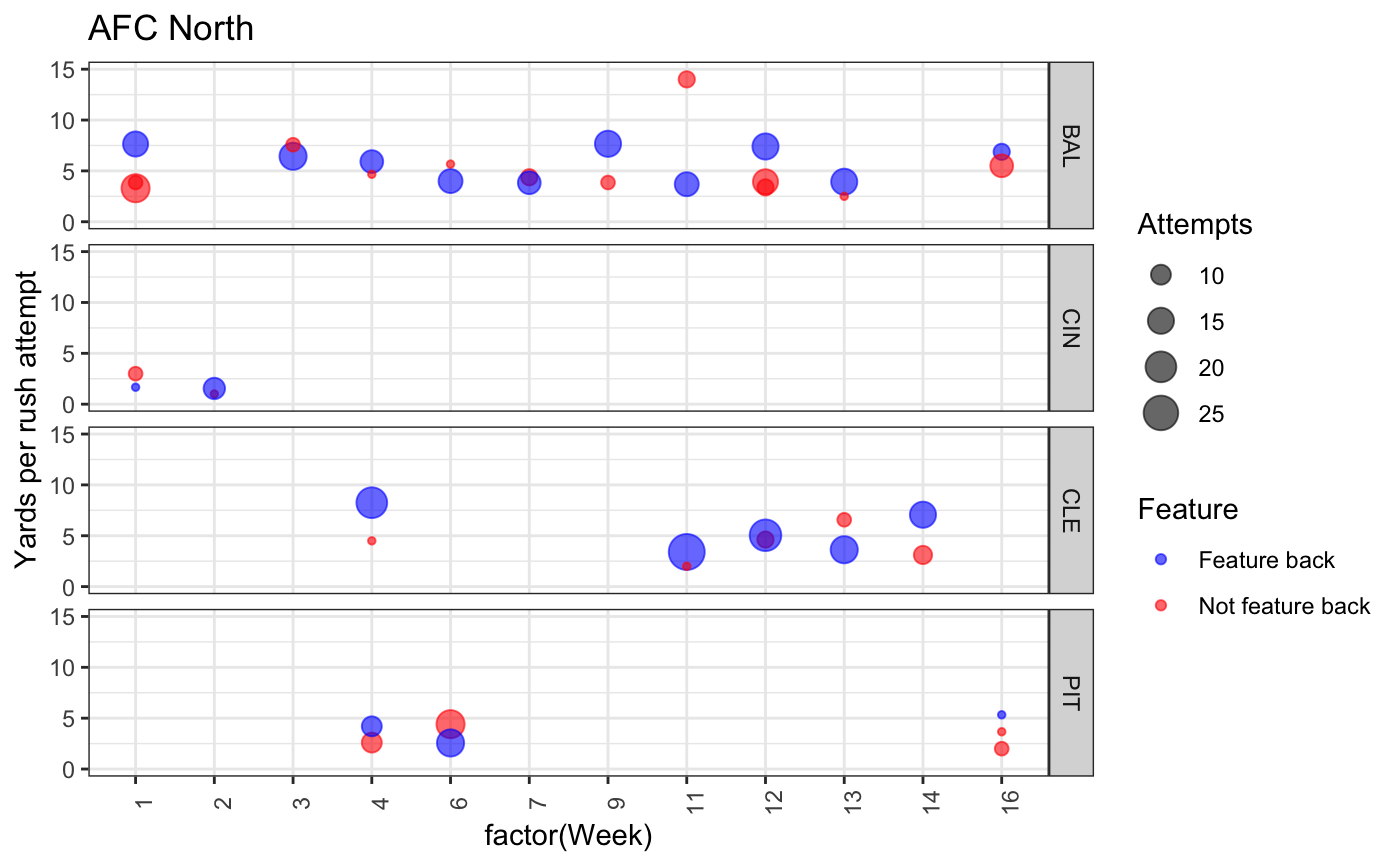
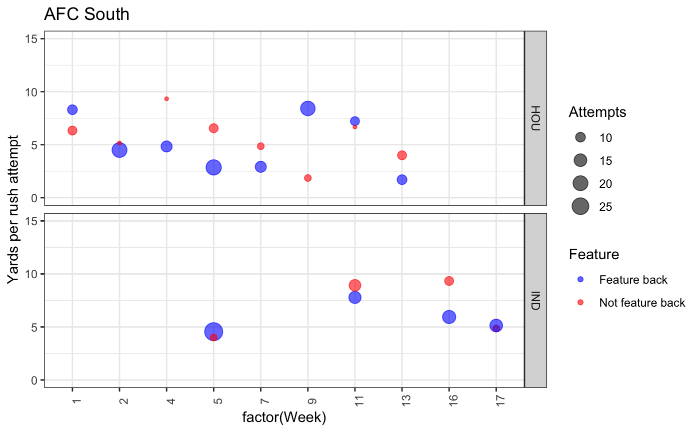
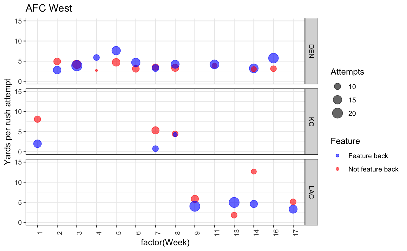
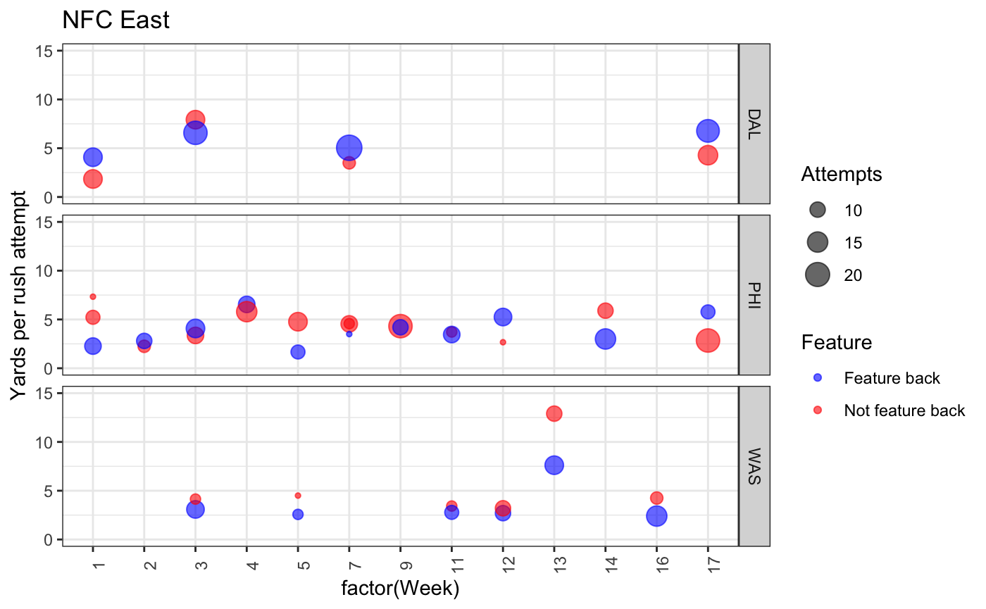
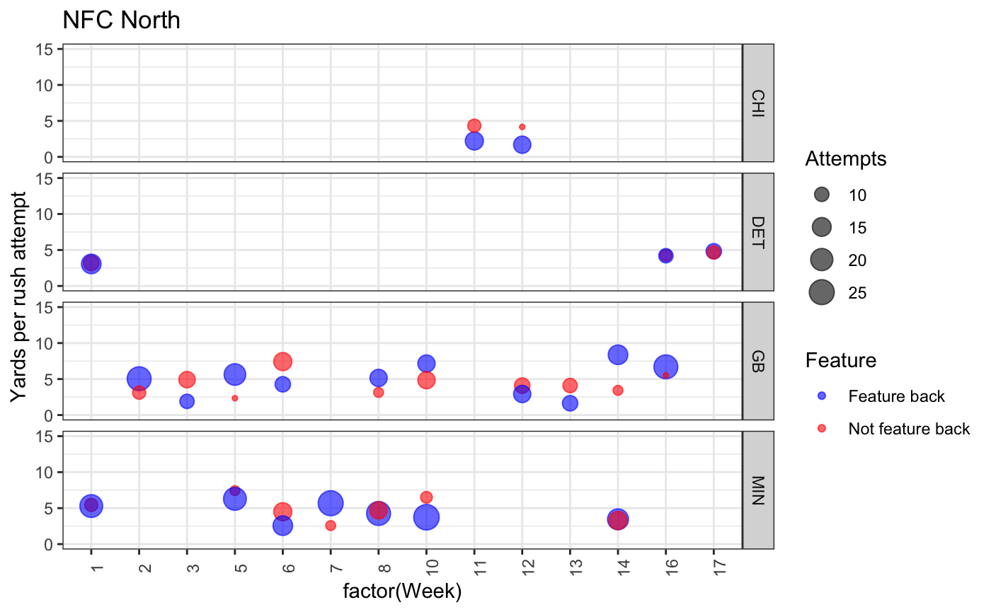
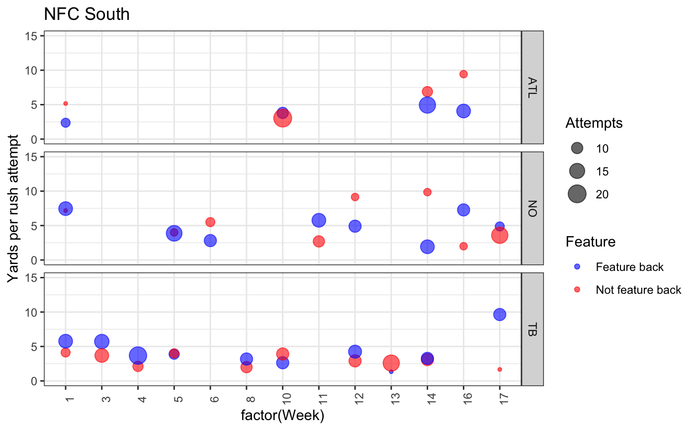
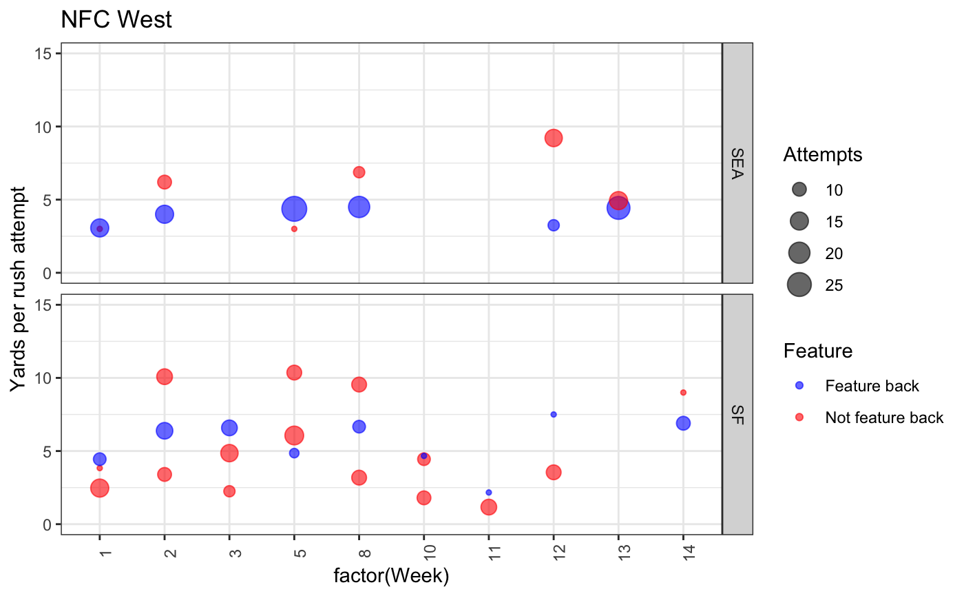
And while these graphs gave me a way to look at all yards per rush attempts in games where a player received 5 carries, my data cleaning was not done yet. Namely, I needed to narrow the dataset down to only the games where both a feature back and not feature back had 5 carries. After doing this, I then replotted this and these results can be found by division for the sake of space below. Also worth noting, I used dots in this case and the dots are sized by the number of carries that the player received in that game. As you’ll see the yards per carry between the featured backs and the not featured backs are pretty similar within week and the featured back tends to, but does not always, have more rush attempts. Additionally, some teams were dropped at this point as these teams did not have at least one game where a feature back and a not feature back each had 5 carries and only games where this happened were kept.
Ok, but did you run any actual analyses?
After doing all this plotting, I finally got around to running some statistics. While I considered other model types (namely a multilevel model for those that are statistically inclined), I wound up using a linear regression equation.
While linear regression equation might sound fancy, it isn’t really too complex and they’re actually kind of easy to understand so I figured I’d provide a brief primer. If you already know what this is then please feel free to skip to the data itself or if you have no interested in learning about it then please feel free to skip to the final section as that provides a no-data summary of what was found.
For those that are still here, basically, a linear regression equation is the same concept as the y = mx + b equation that some of us learned in back in school. In this equation, b is what your estimate of the outcome (y) would be if x (the variable you care about) is 0. So, a non-football example would be a car that is running and in drive where we treat x as the amount of pressure on the pedal and y as the speed. So, in this instance, when the amount of pressure on the pedal (the x variable)) is 0, the car doesn’t move and the speed (the y variable) is 0. Thus, when x is 0, y is 0 and, because this y is 0, b is equal to 0. Building on that, the m is just how much faster the car goes for every 1 bit of force more we put on the pedal. So, in this instance if every 1 bit of force adds 2 miles per hour then m would be equal to 2. Then using this equation, we could calculate our best estimate of how fast a car is going based on the amount of pressure on the pedal. So, if 20 units of pressure is on the pedal then we’d estimate the car is going 40 miles per hour because the y = mx + b equation would be y = 20*2 + 0, which equals 40.
Now the big difference in the data that I’m running and the car example is that I’m just going to have more x’s and more associated m’s, but the concepts are basically all the same.
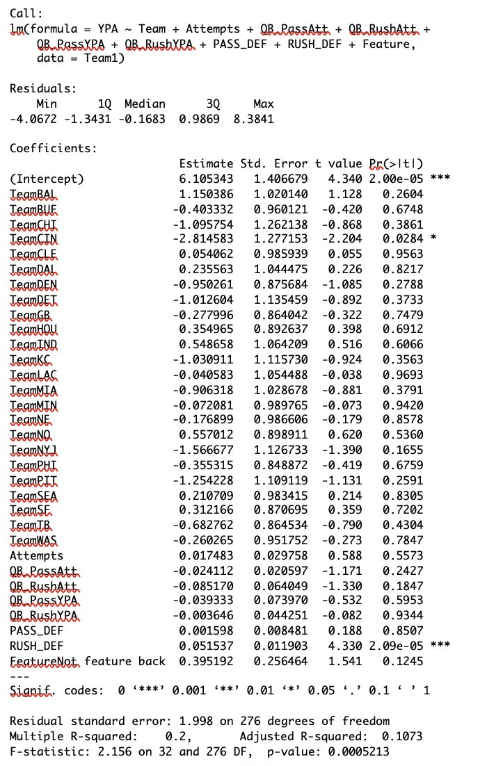
With all of that said, I then ran a model that would predict yards per rushing attempt using the following variables:
And what did the results show?
Based on the 2020 season exclusively, and only using games where a feature back (a player who led the team in carries) and at least one non-feature back had at least 5 rushing attempts, the data did not support that feature backs were more productive as measured exclusively by yards per rush attempt. In general, of the variables that I measured, only team (in some instances such as Cincinnati) and rush defense were predictive of rushing yards on a per carry basis.
With that said rush defense by opposition was really important. As I said earlier, a more negative grade there meant a better grade. So, in this instance, the m, or the beta weight, when x was rush defense grade was .05 and it was statistically significant, which really just means that the data is mostly sure that the m is not actually equal to 0. The best estimate of the m for this variable was .05 which means that for each +1% change in a team’s rush defense as measured by Football Outsiders DVOA, the yards per carry increased by .05. Given that the range between the worst DVOA (18.6) and the best (-33.5) was 49.1, this means that estimate in the yards per rush attempt for a running back who faced the best defense would be 2.45 yards less than the running back who faced the worst run defense, which is a huge difference.
Additionally, if we use a less stringent p value cutoff compared to the “commonly used but based on nothing in reality of .05” then it looks like feature backs may actually do worse than their non-feature back teammates by about .40 yards per carry, but. given that it wasn’t “significant,” I don’t care to read into it too much and would instead conclude that featured and non-featured backs don’t differ much, if at all, on rush yards per attempt after taking into account these other features of the game
So taken together, what really seems to matter in predicting yards per attempt for a given week is simply the team one is on and the defense that they’re facing. The guy actually taking the ball may matter to some degree (albeit the evidence does not support that in this case), but if it does, then the data would better support that the backups are averaging more yards per carry, which is not what we’d expect if starting running backs are meaningfully more talented than their backups.
The exact data that was found can be seen here:
Did you do anything else?
After looking at the data, I had concerns that I wasn’t adequately gauging the value of top-tier running backs. Namely, the above data looks at all teams, which is going to encompass some teams where there’s a true “feature” back like Dallas with Zeke or the Jets with Bell but also teams where there is more of a “running back by committee” approach such as the Bills with Gore and Singletary. Given that, I re-ran the data using the cutoff of 240 carries rather than simply leading the team in carries. Using this cutoff, the final running back included was David Montgomery who ranked 13th in carries in the NFL last season. It was my thought that by using this more stringent requirement to differentiate the “talented” featured running backs and their “less talented” backups then I would be able to better capture how much better the top running backs did than their backups. Unfortunately, after all these whittling downs, the dataset became rather small, which means that it is harder to detect statistical significance, which is relevant for the eventual interpretation.
With that said, I still ran the data using the same rules as laid out previously (namely that they had to have played in a game where the lead back and a backup each had 5 carries.) Using this criteria, the following teams and “Top Running Backs” made the final cut:
-
Teams: CHI, CIN, CLE, DAL, HOU, IND, MIN, NYJ, SEA -
Feature backs: David Montgomery, Joe Mixon, Nick Chubb, Ezekiel Elliott, Carlos Hyde, Marlon Mack, Dalvin Cook, Le’Veon Bell, Chris Carson
Worth nothing, this list is probably not a perfect list of the 9 best running backs, but I think it’s pretty close. We miss out on Christian McCaffrey, Derrick Henry, and Saquan Barley, but I still think that these 9 running backs are clearly perceived as being a few talent notches above their backups, so I think it’s an adequate, if not perfect, data sample.
Once again, before running any analyses, I plotted the points. As you’ll see, the points on a game-by-game basis are often nearly overlapping between the “elite” backs and their backups, which is in line with what we found before.
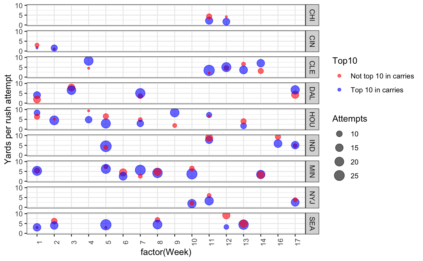
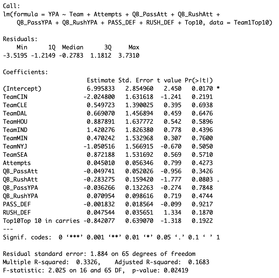
After creating the plots, I then ran the exact same analyses as before, except I used this new top 10 in carries variable rather than the previously used feature back variable
While the “significance values” differ due to the smaller dataset, the estimates are rather similar to before. Namely, rush defense DVOA again has an estimate of .05 and the players that led their team in carries were estimated as averaging less yards per carry. While these values were not significant in this case, they appear to align with the previous analysis and, thus, I give them a bit more weight than I normally do with non-significant values.
What does it all mean?
In summary, it doesn’t appear that different running backs on the same roster generate significantly different yards per rush attempts during the same game against the same defense. So given that, the data does not support paying running backs a ton of money if the goal is to maximize yards per rush attempt because the starters and the backups seem to generate approximately the same yards per rush attempt. This is especially relevant when one considers that top running backs can make 10+ million a plus (see Le’Veon Bell), while their backs ups can often be acquired for amounts close to the veteran minimum of less than 1 million a year (see Bilal Powell and his contract worth $1,020,000).
So, at least in 2020, using these exact analyses, the data does not support that running backs matter.
If anyone has any questions about what I did, what I found, or really anything, please let me know and I’d be happy to answer them
This is a FanPost written by a registered member of this site. The views expressed here are those of the author alone and not those of anybody affiliated with Gang Green Nation or SB Nation.
