A brain network supporting social influences in human decision-making

Choice model specifications. In all models, Choice 1 was accounted for by the option values of option A and option BVt=[Vt(A),Vt(B)](3)where V_t indicated a two-element vector consisting of option values of A and B on trial t. Values were then converted into action probabilities using a Softmax function (5). On trial t, the action probability of choosing option A (between A and B) was defined as followsPt(A)=eVt(A)eVt(A)+eVt(B)=11+e−(Vt(A)−Vt(B))(4)

For Choice 2, we modeled it as a “switch” (coded as 1) or a “stay” (coded as 0) using a logistic regression. On trial t, the probability of switching given the switch value was defined as followsPt(switch)=Φ(Vt(switch))(5)where Φ was the inverse logit linking functionΦ(x)=11+e−x(6)

Note that, in model specifications of the action probability, we did not include the commonly used inverse Softmax temperature parameter τ. This was because we explicitly constructed the option values of Choice 1 and the switch value of Choice 2 in a design-matrix fashion (e.g., Eq. 8; see the text below). Therefore, including the inverse Softmax temperature parameter would inevitably give rise to a multiplication term, which, as a consequence, would cause unidentifiable parameter estimation (24). For completeness, we also assessed models with the τ parameter, and they performed consistently worse than our models specified here.

The category 1 models (M1a, M1b, and M1c) did not consider any social information. In the simplest model (M1a), a Rescorla-Wagner model was used to model the Choice 1, with only the chosen value being updated via the RPE (δ), and the unchosen value remaining the same as the last trial.δchosen,C2,t=Rt−Vchosen,C2,tVchosen,C2,t+1=Vchosen,C2,t+αδchosen,C2,tVunchosen,C2,t+1=Vunchosen,C2,t(7)where R_t was the outcome on trial t and α (0 < α < 1) denoted the learning rate that accounted for the weight of RPE in value update. A β weight (β_V) was then multiplied with the values before being submitted to Eq. 4 with a categorical distribution, as inC1t∼Categorical(Softmax(βvVt))(8)

Because there was no social information in M1a, the switch value of Choice 2 was composed merely of the value difference of Choice 1 and a switching bias (i.e., intercept)Vt(switch)=βbiasC2+βvdiffC2(Vchosen,C1,t−Vunchosen,C1,t)(9)

Choice 2 was then modeled with this switch value following a Bernoulli distributionC2∼Bernoulli(Vt(switch))(10)

In M1b, we tested whether the fictitious update could improve the model performance, as the fictitious update has been successful in PRL tasks in nonsocial contexts (20, 27). In M1b, both the chosen value and the unchosen value were updated, as inδchosen,C2,t=Rt−Vchosen,C2,tδunchosen,C2,t=−Rt−Vunchosen,C2,tVchosen,C2,t+1=Vchosen,C2,t+αδchosen,C2,tVunchosen,C2,t+1=Vunchosen,C2,t+αδunchosen,C2,t(11)

In M1c, we assessed the Pearce-Hall (45) model that entailed a dynamic learning rateδchosen,C2,t=Rt−Vchosen,C2,tVchosen,t+1=Vchosen,t+kαtδchosen,C2,tVunchosen,C2,t+1=Vunchosen,C2,tαt+1=λ∣δchosen,t∣+(1−λ)αt(12)where k (0 < k < 1) was the weight of the (dynamic) learning rate and λ (0 < λ < 1) indicated the weight between RPE and the learning rate.

Our category 2 models (M2a, M2b, and M2c) tested the role of instantaneous social influence on Choice 2, namely, whether observing choices from the other coplayers contributed to the choice switching. As compared with M1 (M1a, M1b, and M1c), only the switch value of Choice 2 was modified, as followsVt(switch)=βbiasC2+βvdiffC2(Vchosen,C1,t−Vunchosen,C1,t)+βagainstw.Nagainst,t(13)where w.N_against,t denoted the preference-weighted amount of dissenting social information relative to each participant’s Choice 1 on trial t. It was computed on a trial-by-trial fashion as followsw.Nagainst,t=∑s=1Kws,t∑s=14ws,t,K=0,1,…,4(14)where K indicated the number of opposite choices from the others and w_s,t was participants’ trial-by-trial preference weight toward the other four coplayers. Note that these preference weights were fixed parameters based on each participant’s preference toward the others when uncovering their choices: The first favored coplayer received a weight of 0.75, the second favored coplayer received a weight of 0.5, and the remaining two coplayers received a weight of 0.25, respectively. They were not modeled as free parameters because doing so caused unidentifiable model estimate behavior. All other specifications of models in this category (M2a, M2b, and M2c) were identical to models in category 1 (M1a, M1b, and M1c), respectively.

Our category 3 models (M3, M4, M5, M6a, and M6b) assessed whether participants learned from their social partners and whether they updated vicarious option values through social learning. Note that models belonging to category 2 solely considered the instantaneous social influence on Choice 2, whereas models in category 3 tested several competing hypotheses of the vicarious valuation that may contribute to Choice 1 on the following trial, in combination with individuals’ own valuation processes. In all models within this category, the option values of Choice 1 were specified by a weighted combination between V_self updated via direct learning and V_other updated via social learningVt=βvselfVself,t+βvotherVother,t(15)whereVself,t=[Vself,t(A),Vself,t(B)]Vother,t=[Vother,t(A),Vother,t(B)](16)

Note that given that M2b was the winning model among category 1 and category 2 models (Table 1), we used M2b’s specification for the value update of V_self (Eq. 11), so that category 3 models only differed on the specification of V_other.

M3 tested whether individuals recruited a similar RL algorithm to their own when learning option values from observing others. Hence, M3 assumed participants to update values “for” the others using the same fictitious update rule for themselvesδs,chosen,C2,t=Rs,t−Vs,chosen,C2,t,s=1,2,3,4δs,unchosen,C2,t=−Rs,t−Vs,unchosen,C2,tVs,chosen,C2,t+1=Vs,chosen,C2,t+αoδs,chosen,C2,tVs,unchosen,C2,t+1=Vs,unchosen,C2,t+αoδs,unchosen,C2,t(17)where s denoted the index of the four other coplayers and α_o was the learning rate for the others. These option values from the four coplayers were then preference-weighted and summed to formulate V_other, as followsVother,t+1(A)=∑s=14ws,tVs,t+1(A)Vother,t+1(B)=∑s=14ws,tVs,t+1(B)(18)where w_s,t was participants’ preference weight. To ensure that the corresponding value-related parameters (β_vself and β_vother in Eq. 15) were comparable, V_other was further normalized to lie between −1 and 1 with the Φ(x) function defined in Eq. 6Vother,t+1(A)=2Φ(Vother,t+1(A))−1Vother,t+1(B)=2Φ(Vother,t+1(B))−1(19)

One may argue that having four independent RL agents as in M3 was cognitively demanding: To accomplish so, participants had to track and update each other’s individual learning processes together with their own valuation (together 2⁵ units of information). We, therefore, constructed three additional models that used simpler but distinct pathways to update vicarious values via social learning. In essence, M3 considered both choice and outcome to determine the action value. We then asked whether using either choice or outcome alone may perform well as, or even better than, M3. Following this assumption, we constructed (i) M4 that updated V_other using only the others’ action preference, (ii) M5 that considered the others’ current outcome to resemble the value update via observational learning, and (iii) M6a that tracked the others’ cumulative outcome to resemble the value update via observational learning.

In M4, other players’ action preference (ρ) is derived from the choice history over the last three trials using the cumulative distribution function of the beta distribution at the value of 0.5 (I_0.5). That isρs,t(A)=I0.5(1+∑t=T−2TC2B,s,t,1+∑t=T−2TC2A,s,t)ρs,t(B)=1−ρs,t(A)(20)where s denoted the index of the four other coplayers and t denoted the trial index from T − 2 to T. To illustrate, if one coplayer chose option A twice and option B once in the last three trials, then the action preference of choosing A for him/her was as follows: I_0.5(frequency of B + 1, frequency of A + 1) = I_0.5(0.5, 1 + 1, 2 + 1) = 0.6875. V_other was computed on the basis of these action preferencesVother,t+1(A)=∑s=14ws,tρs,t(A)Vother,t+1(B)=∑s=14ws,tρs,t(B)(21)where w_s,t was participants’ preference weight and s denoted the index of the four other coplayers. Similar to M3, the computation of V_other here was also preference-weighted and summed. The values were similarly normalized using Eq. 19.

By contrast, M5 tested whether participants updated V_other using only each other’s reward on the current trial, which was equivalent to the standard Rescorla-Wagner model with α = 1, indicating no trial-by-trial learningVother,t+1(A)=∑s=1KAws,tRs,t,KA=0,1,…,4Vother,t+1(B)=∑s=14−KAws,tRs,t(22)where w_s,t was participants’ preference weight, s denoted the index of the four other coplayers, t denoted the trial index from T − 2 to T, and K_A denoted the number of coplayers who decided on option A on trial t. Similar to M3, the computation of V_other here was also preference-weighted and summed. These values were then normalized using Eq. 19.

Moreover, M6a assessed whether participants tracked cumulated reward histories over the last few trials instead of monitoring only the most recent outcome of the others. A discounted reward history over the recent past (e.g., the last three trials) has been a relatively common implementation in other RL studies in nonsocial contexts (22, 46). By testing four window sizes of trials (i.e., two, three, four, or five) and using a nested model comparison, we decided on a window of three past trials to accumulate the other coplayers’ performanceVother,t+1(A)=∑s=1KA∑t=T−2Tws,tγT−iRs,i,KA=0,1,…,4Vother,t+1(B)=∑s=14−KA∑t=T−2Tws,tγT−iRs,i(23)where γ (0 < γ < 1) denoted the rate of exponential decay and all other notions were as in Eq. 22. Similar to M3, the computation of V_other here was also preference-weighted and summed. The values were then normalized using Eq. 19.

Last, given that M6a was the winning model among all the models above (M1 to M6a) indicated by model comparison (see below model selection; Table 1), we further assessed in M6b whether Bet 1 contributed to the choice switching on Choice 2, as followsVt(switch)=βbiasC2+βvdiffC2(Vchosen,C1,t−Vunchosen,C1,t)+βagainstw.Nagainst,t+βbet1Bet1t(24)

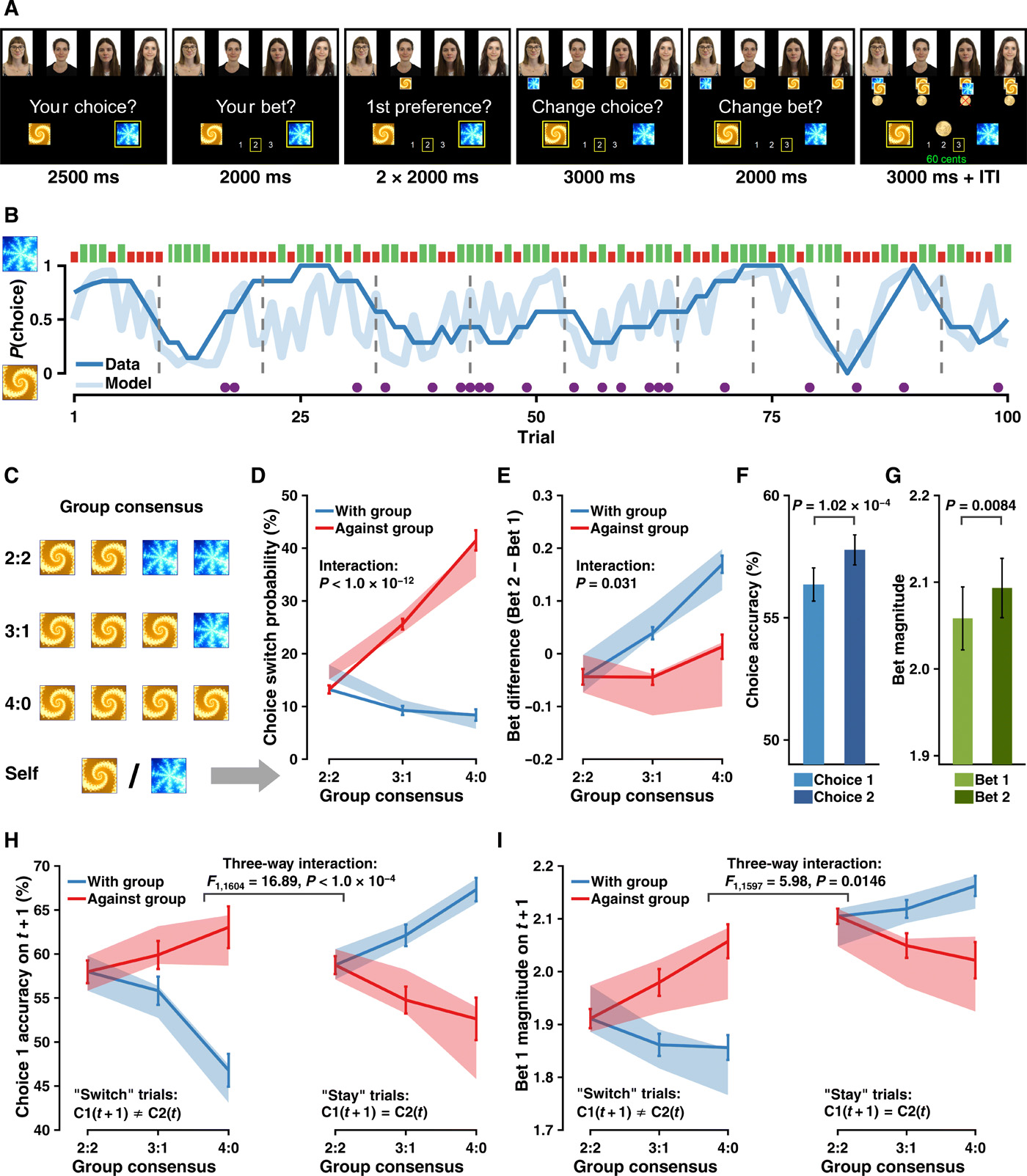
Note that in M6a/M6b, V_other differed from V_self in practice. On trial t, V_self of a punished option might largely decrease given the negative RPE, whereas V_other may not be vastly affected because of the others’ previous successes [e.g., V_other(blue); Fig. 2C; albeit a loss on trial t, the cumulative reward history was still positive, indicating that the cumulative performance was still reliable]. Both V_self and V_other spanned within their range (−1 to 1; Fig. 2D) with a slightly moderate correlation (r = 0.38 ± 0.097 across participants; Fig. 3A), and they jointly contributed to the action probability of Choice 1.

Bet model specifications. In all models, both Bet 1 and Bet 2 were modeled as ordered-logistic regressions that are often used for quantifying ordered discrete variables, such as Likert-scale questionnaire data (24). We applied the ordered-logistic model because the bets in our study indeed inferred an ordinal feature. Namely, betting on three was higher than betting on two, and betting on two was higher than betting on one, but the difference between the bets of three and one (i.e., a difference of two) was not necessarily twice as the difference between the bets of three and two (i.e., a difference of one). Hence, we sought to model the distance (decision boundary) between them. Moreover, we hypothesized a continuous computation process of bet utilities when individuals were placing bets, which satisfied the general assumption of the ordered-logistic regression model.

There were two key components in our bet models, the continuous bet utility U_bet and the set of boundary thresholds θ. Specifically, the bet utility U_bet varied between K − 1 thresholds (θ_{1,2, …, K−1}) thresholds to predict bets. Since there were three bet levels in our task (K = 3), we introduced two decision thresholds, θ₁ and θ₂ (where θ₂ > θ₁). Hence, the predicted bets (bêt) on trial t were represented as followsbêti,t={1,if−∞<Ubeti,t<θ12,if θ1<Ubeti,t<θ2,i=1,23,if θ2<Ubeti,t<+ ∞(25)where i indicated either Bet 1 or Bet 2. Because there were only two levels of threshold, for simplicity, we set θ₁ = 0 and θ₂ = θ (where θ > 0). To model the actual bets, a logistic function (Eq. 6) was used to obtain the action probability of each bet, as follows{P(beti,t=1)=Φ(−Ubeti,t)P(beti,t=2)=Φ(θ−Ubeti,t)−Φ(−Ubeti,t),i=1,2P(beti,t=3)=1−Φ(θ−Ubeti,t)(26)

The utility U_bet1 was composed of a bet bias and the value difference between the chosen option and the unchosen optionUbet1,t=βbiasB1+βvdiffB1(Vchosen,C1,t−Vunchosen,C1,t)(27)

The rationale was that the larger the value difference between the chosen and the unchosen options, the more confident individuals were expected to be, hence placing a higher bet. This utility U_bet1 was kept identical across all models (M1a to M6b), and Bet 1 was modeled as followsB1t∼OrderedLogistic(Ubet1,t∣θ)(28)

In addition, Bet 2 was modeled as the bet change relative to Bet 1. Therefore, the utility U_bet2 was constructed on the basis of U_bet1. In all nonsocial models (M1a, M1b, and M1c), the bet change term was represented by a bet change bias (i.e., intercept), depending on whether participants had a switch or stay on their Choice 2Ubet2,t={Ubet1,t+βbiasstay,if C1=C2Ubet1,t+βbiasswitch,if C1≠C2(29)

In all social models (M2a to M6b), regardless of the observational learning effect, the bet change term was specified by the instantaneous social information together with the bias, depending on whether participants had a switch or stay on their Choice 2Ubet2,t={Ubet1,t+βwithstayw.Nwith,t+βagainststayw.Nagainst,t,if C1=C2Ubet1,t+βwithswitchw.Nwith,t+βagainstswitchw.Nagainst,t,if C1≠C2(30)withw.Nagainst,t=∑s=1Kws,t∑s=14ws,t,K=0,1,…,4w.Nwith,t=∑s=14−Kws,t∑s=14ws,t(31)where K indicated the number of opposite choices from the others and w_s,t was participants’ trial-by-trial preference weight toward the other four coplayers. Note that, however, despite the high negative correlation between w.N_with and w.N_against, the parameter estimation results showed that the corresponding effects (i.e., β_with and β_against) did not rely on each other (r = 0.04, P > 0.05). As shown in Fig. 2H, the corresponding parameters showed independent contributions to bet changes during the adjustment. In addition, we constructed two other models using either w.N_with or w.N_against alone, but both models’ performance markedly reduced than including both of them [∆LOOIC (leave-one-out information criterion relative to the winning model) > 1000]. Last, the utility U_bet2 was kept identical across all social models (M2a to M6b), and Bet 2 was modeled as followsB2t∼OrderedLogistic(Ubet2,t∣θ)(32)